Does Your Neighbor Being Muslim Make You More Muslim: Investigating the Spatial Auto-Correlation of Culture

The paper was written for a class in my MPAI/ID program called “Spatial Models for Social and Environmental Policy.”

Does Your Neighbor Being Muslim Make You More Muslim: Investigating the Spatial Auto-Correlation of Culture

I. Introduction and Context

This paper seeks to investigate the spatial auto-correlation of culture. Taking Islam as a form of culture, this paper asks if countries are more likely to be more Muslim if they are surrounded by more Muslim neighboring countries. I build on research by Michalapoulos, Naghavi and Prarolo (2012) who undertake an economic history based analysis to determine what makes a country more or less likely to be Muslim. Specifically, I undertake spatial regressions to see if a country’s ‘Muslim-ness’, as defined by the proportion of people in the country who identify themselves as Muslim, is also associated with the ‘Muslim-ness’ of its neighboring countries. I find that the ‘Muslim-ness’ of nations is statistically significantly spatially auto-correlated and models that account for spatial auto-correlations do a better job of fitting the data than ones that do not.

The field of cultural economics is nascent, though it has been expanding rapidly in recent years. In essence, cultural economics is the causal quantification of historical or contemporary cultural traits – based on theories from other fields in the social sciences such as anthropology, sociology and psychology – on socio-economic outcomes today. Before providing examples of such research in the field of cultural economics, it would be first useful to define what ‘culture’ is, for the sake of clarity and consistency. I take the definition provided by Guiso, Sapienza and Zingales (2006) which defines culture as “…those customary beliefs and values that ethnic, religious, and social groups transmit fairly unchanged from generation to generation.”

So, how does culture impact economic outcomes? Consider research by Alesina, Giuliano and Nunn (2013) which shows that societies that have a history of plough agriculture tend to exhibit more gender unequal attitudes today. The plough technology enabled division of labor in agriculture with men being more likely to tend to the fields while women engaged in domestic work in the homes. This thereby led to different gender attitudes (culture) which persist till today. One of the more astonishing findings in this paper is that second generation migrants tended to exhibit the gender attitudes of their ‘home’ culture rather than the culture of their new nation, showing that the channel through which gender attitudes persist is culture, as opposed to surroundings. Other examples of research along these lines include Nunn and Wantchekon (2011) who show that current differences in trust levels within Africa can be traced back to the transatlantic and Indian Ocean slave trades. In addition, Greif (2006) discusses cultural differences between Maghribi and Genoese traders that led to different de jure versus de facto legal systems in the Muslim Mediterranean and Venice respectively.

Diving more deeply into a particular branch of culture, this paper focuses on the impact of religion on national outcomes. The notion that religion can have important effects on social, economic and political outcomes has historically been one of deep interest, as evidenced by pioneering work by Max Weber (1905) who argued that Protestant societies were more likely to experience better economic outcomes because the Protestant ethic was embodied among the people in those societies. While this formulation has been challenged, for instance, by Becker and Woessmann (2009) who argue that it was rather the human capital channel – where Protestants had to learn to be literate as they had to learn to read the Bible – that led to more prosperous economies, the general sentiment still holds – religion, or aspects pertaining to religion, can lead to important social, political and economic outcomes. For instance, Barro and McCleary (2006) provide a helpful overview of the two-way relationship between religion and economic growth. This is corroborated by Guiso, Sapienza and Zingales (2003) who find that, on average, religious beliefs are associated with economic attitudes that are conducive to higher per capita income and growth.

Despite the growing amount of literature on cultural economics, what has been sorely missing from the discussion has been the spatial distribution of culture. Put simply, is culture spatially correlated? The reason that this is important, particularly from a research perspective, is that culture as a variable in econometric analysis is often instrumented by some other variable in a Two Stage Least Squares (2SLS) regression. A 2SLS approach requires finding a credible ‘instrument’ – one that impacts the dependent variable only via the independent variable of interest (exclusion restriction). Well-known instruments in the field include settler mortality for Acemoglu, Johnson and Robinson (2001), type of soil for Alesina, Giuliano and Nunn (2013), and change in rainfall for Miguel, Satyanath and Sergenti (2004).

However, notice that for all these instruments, there is a possibility that spatial autocorrelation exists. For instance, if the disease environment is particularly hostile to foreign colonists in country A, is it not also more likely that the disease environment be hostile to foreign colonists in neighboring country B? After all, mosquitoes do not recognize borders. If spatial autocorrelation exists in the instrument, then there is a possibility of unaccounted for spatial autocorrelation in the independent variables (cultural variables) and potentially even the dependent variable. Thus, we can then ask if the independent variable – culture – is something that is spatially autocorrelated and if it is, how do we ensure it is well-accounted for in econometric specifications?

This paper is a first attempt at answering that question, using religion as a branch of culture to investigate if more Muslim neighboring nations are associated with a home nation’s Muslim-ness. I find that, indeed, ‘Muslim-ness’ is spatially auto-correlated and that a failure to account for spatial auto-correlations lead to mis-specified and inaccurate models of ‘Muslim-ness’ determination. The paper is organized as follows. Section II discusses the data and methodology of this study, while Section III discusses the results of the analyses. Section IV reviews the caveats to the analysis, concludes and provides policy implications.

II. Data and Methodology

Data for ‘Muslim-ness’ is taken from the Correlates of War (“COW”) Project. The Correlates of War Project was founded in 1963 by J. David Singer, a political scientist at the University of Michigan. The project’s purpose is to systemically accumulate scientific knowledge about war and does so by facilitating the collection, dissemination and use of accurate and reliable quantitative data in international relations. The unit analysis for all data in the Correlates of War Project is the ‘state’. Available data from the Correlates of War project includes The New COW War Data, 1816-2007, which provides a list of wars from 1816 to 2007, National Material Capabilities which gives six indicators that determine state power, Diplomatic Representation between countries from 1817 to 2005 and Bilateral Trade flows between states from 1870 to 2009, among others.

For the purposes of this paper, I take the Correlates of War project’s World Religion Data which provides detailed information about religious adherence worldwide, in 5-year intervals, from 1945 to 2010. The data records percentages of the state’s population that practice a given religion. Religions included in this data set are, among others, Christianity, Judaism, Islam, Buddhism, Hinduism and, even, Atheism. All data are collated from the respective nations’ statistical databases such as censuses, surveys, fact-books and so on. With this data, I define the degree of ‘Muslim-ness’ of a country as the historical 55-year average percentage of population that is Muslim. This definition is useful on several counts. Firstly, it allows for the ‘depth’ of historical Muslim-ness in a country which allows for greater variation across states and thus, better empirical estimates of gender attitudes as opposed to a simple binary configuration. Secondly, if culture, as defined by Guiso, Sapienza and Zingales (2006) as something that is transmitted from generation to generation, then taking the long-run ‘Muslim-ness’ of a country may proxy how more deeply-ingrained Islam is in the present culture of the given country. There is some caution on taking the mean percentage of the Muslim population especially with regards to countries with high variances, but it is unlikely that, except in the event of exodus and/or genocide, the proportion of Muslims in a country would have a high standard deviation.

To predict the Muslim-ness of a country, I build on the hypothesis by Michalapoulos, Naghavi and Prarolo (2012). Their paper examines the spatial distribution of Muslim societies, attempting to shed light on the geographic origins of Muslim societies. Their empirical analysis was conducted across nations, ‘virtual nations’ and ethnicities and establishes that geographic inequality and proximity to pre-Islamic trade routes are key factors that explain present-day Muslim adherence.

The hypothesis that proximity to trade routes, even long-distance trade routes, was critical in the expansion of Islam is well-documented by prominent Islamic scholars; further references are available in Michalapoulos, Naghavi and Prarolo (2012). However, according to the authors, the tight relationship between geographic inequality and Muslim adherence is less well-known. They argue that a region that is characterized by unequal agricultural potential implies that there are few pockets of arable land where farming is feasible and a large share of dry regions where pastoralism is the most likely economic activity. These differences enable people living in those areas to specialize, which provided the basis for intra-regional trade. The next way in which unequal geography led to the expansion of Islam is the linkage between geographic inequality and social inequality and predation within a region. The authors point out that Ibn Khaldun, one of the most important philosophers in both the Muslim and world history, observed that a crucial factor for understanding Muslim history is “the central social conflict between the primitive Bedouin and the urban society.” Nomads posed a threat to lands which were highly arable for farming. To combat this, the authors argue that Islam provided a centralizing state-building force, featuring redistributive principles, which enabled order and relative peace in the region, thereby further facilitating trade and inducing Islamic culture.

However, their paper makes no note of whether spatial correlation in the error terms – thereby the spatial auto-correlation of ‘Muslim-ness’ – matters. While they conduct OLS regressions and several robustness checks to establish their claim, they do not undertake a spatial errors regression or spatial lags regression. Therefore, this project attempts to enhance their analysis by accounting for spatial auto-correlation.

To set the baseline for studying the spatial auto-correlation of culture – in this case, the spatial auto-correlation of Muslim-ness – I first undertake a standard OLS regression, as follows:-

Islami = β1GeogInequalityi + β2DistanceTradei + ε (1)

Islami represents the Muslim-ness of country i from 1945 to 2010. GeogInequalityi represents the geographic inequality, as defined by Michalapoulos, Naghavi and Prarolo (2012), for country i while DistanceTradei represents the distance of country i from the pre-Islamic trade routes. If Michalapoulos, Naghavi and Prarolo (2012) are right, then β1 and β2 should be statistically significantly positive and negative respectively. ε is the error term.

To check if the errors are spatially correlated, I undertake a Local Moran’s I test of the residuals. If ‘Muslim-ness’ is not spatially auto-correlated, then we should expect to see no spatial correlation of the residuals and thus, a Moran’s I coefficient that is close to zero.

To investigate further, I undertake two forms of spatial regression analysis. The first model is the spatial lag model, which includes a spatial lag variable in the right hand side of the equation. I use a Queen’s Contiguity weight of order 2. This means that the spatial weight used for the regression is based on the Muslim-ness of a given country’s neighbors that are 2 orders away. For instance, the Muslim-ness of Singapore is weighted not just by the Muslim-ness of Malaysia, but also of Thailand. The spatial lag variable controls for the Muslim-ness of the neighbors. The specification is as follows:-

Islami = ρWIslamj(i) + β1GeogInequalityi + β2DistanceTradei + ε (2)

W represents the weightage used in the regression while Islamj(i) represents the spatial lag of the dependent variable, or in other words, the Muslim-ness of i’s neighbors. If ‘Muslim-ness’ is spatially auto-correlated, then we expect the weighted coefficient on Islamj(i) to be statistically significant. To check if the specification improves on the OLS model, I undertake a Local Moran’s I test of the residuals and I check to see if the Log likelihood and R-squared of the regression increase vis-à-vis the OLS specification.

To further sharpen the analysis, I also undertake a spatial errors regression. In this regression, spatial effects are incorporated through the error term, ε. The error term is estimated by taking into account both the spatially weighted errors and the non-spatially auto-correlated errors and thus, including the error term into the main regression means that spatial auto-correlation is controlled for in the model. The specification is as follows:-

Islami = β1GeogInequalityi + β2DistanceTradei + ε (3)

where ε = λWε + κ (4)

λ represents the coefficient on the spatial auto-correlation of the errors – how much is the error term impacted by the error term of the country’s neighbors – while k represents the vector of errors that are not spatially auto-correlated. Similar to the above, I undertake a Local Moran’s I test of the residuals and I check to see if the Log likelihood and R-squared of the regression increase vis-à-vis the OLS specification and the Spatial Lag specification. The results are reported in Section III.

III. Results and Discussion

There are 113 observations from the merged datasets. I begin with a preliminary overview on whether Islam is spatially auto-correlated. This motivates the need to move from standard OLS regressions to ones which control for potential spatial auto-correlation, such as the spatial lag and spatial error regressions. Figure 1 in the Appendix shows the LISA Cluster Map for ‘Muslim-ness’ of nations. The map shows the results of the Univariate Local Moran’s I calculation for ‘Muslim-ness.’ As we can see, there are statistically significant High-High clusters of ‘Muslim-ness’ particularly in North Africa and the Middle East. In South America, we observe statistically significant Low-Low clusters. In line with this, I find that the Moran’s I coefficient – which calculates the spatial correlation of ‘Muslim-ness’ of nations relative to their neighbors (spatial lags) – to be high at 0.46, as shown in Figure 2. Thus, there is some preliminary evidence to suggest that a nation’s Muslim-ness – our proxy for culture for the purposes of this paper – is spatially correlated with the Muslim-ness of its neighbors.

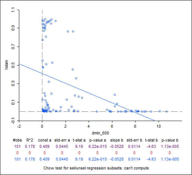
Figures 3 and 5 show the Quintile Maps for the control variables distance from pre-Islamic trade routes and Geographic Inequality respectively. Darker areas on the maps in Figure 3 and Figure 5 indicate greater distance from the pre-Islamic trade routes and greater geographic inequality respectively. Figure 4 shows the scatterplot of ‘Muslim-ness’ versus distance from pre-Islamic trade routes. As predicted by Michalapoulos, Naghavi and Prarolo (2012), there seems to be a negative relationship between distance from the pre-Islamic trade routes and the degree of ‘Muslim-ness’ of a nation. Indeed, the bivariate regression coefficient on pre-Islamic trade route is statistically significantly negative at the 5% level. Figure 6 shows the scatterplot of ‘Muslim-ness’ with geographic inequality. As predicted, higher geographic inequality for a given nation is associated with a higher degree of ‘Muslim-ness’, also statistically significant at the 5% level. Therefore, what these preliminary statistics show is that while Michalapoulos, Naghavi and Prarolo (2012) are likely right in their hypothesis that how Muslim a country is is associated with that country’s distance from the pre-Islamic trade routes as well as its geographic inequality, it is also likely that ‘Muslim-ness’ is spatially auto-correlated. Therefore, a failure to incorporate spatial correlation may lead to mis-specified models. To see if spatial regressions are a better fit for the data at hand, I first consider the standard OLS regression before turning to the Spatial Lag regression and the Spatial Errors regression.

Table 1 displays the results of the OLS regression. As expected, the coefficients on the control variables are of the expected sign and are both statistically significant at the 5% level. The R-Squared of the regression is approximately 0.30 while the Log-Likelihood – both are measures of the fit of the model – is recorded at -28.35. To check if the residuals are spatially auto-correlated, I calculate the Moran’s I statistic of the OLS residuals with respect to the spatially lagged OLS residuals, pictured in Figure 7. The residuals are spatially auto-correlated with a Moran’s I statistic of approximately 0.32. This therefore implies that spatial auto-correlation is present in the dependent variable, the ‘Muslim-ness’ of nations. Using a Local Moran statistic, we see from Figure 8 that there is clustering of the residuals in Europe and in Africa. Thus, an OLS regression would not be the ideal model to explain why some countries are more Muslim than others. We therefore turn to spatial regressions.

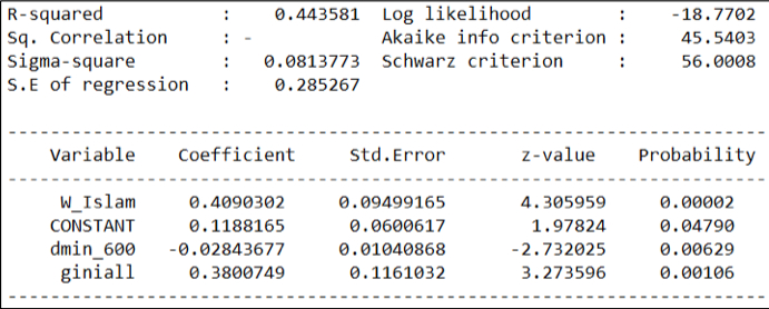
Table 2 shows the Spatial Lag regression specification results. Recall that in the Spatial Lag regression, a regressor that represents the weighted ‘Muslim-ness’ of a given country’s neighbor is added to the right hand side of the regression equation. Like the OLS regression, the coefficients on the control variables are again of the expected sign and are also both statistically significant at the 5% level. However, the magnitude of the coefficients has decreased. This is likely explained by the fact that the coefficient on the spatial lag variable, ρ, is statistically significantly positive at the 5% level. Thus, on average, holding constant distance from pre-Islamic trade routes and geographic inequality, a 10% increase in the proportion of Muslims in a given country’s (second order) neighbors is associated with a 4% increase in the proportion of Muslims in that given country.

The R-Squared of the regression is approximately 0.44 while the log-likelihood is recorded at -18.77. Figure 9 shows the scatterplot of the residuals from the Spatial Lag regression against the spatially lagged residuals. As we can see, the line is now essentially flat, with a Moran’s I statistic of -0.01. This implies that after having controlled for spatial auto-correlation, there is essentially no longer any spatial auto-correlation in the error term. Furthermore, some of the clusters identified by the Local Moran’s analysis in the OLS have disappeared in the Spatial Lag specification, as can be seen in Figure 10. Therefore, it stands to reason that the Spatial Lag regression is a better-fitted model to address the research question and thus, spatial auto-correlation of religion and culture must be taken into account when figuring out why some countries are more Muslim than others.

Next, I try an alternative specification to account for spatial auto-correlation – the Spatial Errors model. Recall that in the Spatial Errors model, spatial auto-correlation is controlled for via estimating the spatial auto-correlation corrected error term. Table 3 shows the results of the Spatial Errors regression. Notice that both geographic inequality and distance from pre-Islamic trade routes are both statistically significantly negative at the 5% level again. However, their magnitude of the coefficients lies somewhere between the magnitudes estimated in the OLS Regression and those estimated in the Spatial Lag regression. λ, the coefficient representing spatial auto-correlation in the error term, is statistically significant at the 5% level, indicating that spatial auto-correlation exists in ‘Muslim-ness’.

The R-Squared of the regression is approximately 0.43 while the log-likelihood is recorded at -20.27. Figure 11 shows the scatterplot of the Spatial Errors residuals versus the spatially lagged residuals. After accounting for spatial auto-correlation, the line is nearly flat, with a Moran’s I coefficient of -0.03. Furthermore, there are fewer clusters in the Local Moran’s analysis in Figure 12 than in the OLS analysis. Thus, the Spatial Errors model is a superior fit to the data relative to the OLS model. In other words, spatial auto-correlation matters.

We have seen that both spatial regression models explain ‘Muslim-ness’ of nations better than does the standard OLS model. The question then becomes – which model do we use? There are several statistics we can use for guidance. The first is the log-likelihood statistic. The larger the statistic (or less negative, in this case), the better the model. Given that the log-likelihood statistic of the Spatial Lag model stands at -18.77 while the log-likelihood statistic of the Spatial Errors model stands at -20.27, it stands to reason that the Spatial Lag model is the better specification to use. Note that we could also consider the R-Squared statistic, but the R-Squared statistics of both specifications are roughly the same. The next statistic we can use for this is displayed in Table 4. Since both the Lagrange Multiplier in the lag and error models are statistically significant, we can consider the robust Lagrange Multipliers. Notice that the Robust Lagrange Multiplier is statistically significant in the ‘lag’ model but is not statistically significant in the ‘error’ model. This implies that in the error model, there exist misspecification problems that invalidate the Robust Lagrange Multiplier test statistic.

Thus, with those statistics in mind, we can advance the Michalapoulos, Naghavi and Prarolo (2012) hypothesis. While distance from pre-Islamic trade routes and geographic inequality matter in relation to the ‘Muslim-ness’ of nations, the analysis of a nation’s ‘Muslim-ness’ would be incomplete without taking into account the spatial auto-correlation of ‘Muslim-ness.’ This paper has shown that the Spatial Lag model – which controls for the weighted ‘Muslim-ness’ of a nation’s neighbors – is a better fit for the data. Thus, we can argue that there exists evidence of spatial auto-correlation of religion and thus, by the Guiso, Sapienza and Zingales (2006) definition, of culture.

IV. Caveats and Conclusion

While the spatial analyses conducted in this paper lends heavy support to the idea that culture – via religion – is spatially auto-correlated, there are several caveats, technical and conceptual, that need to be acknowledged. From a technical perspective, there are over 200 nations in the world, but data, in this paper, is only available for 113 of these. Thus, there is a large amount of missing data, which is likely not by random chance; consider countries in Africa, for instance, where any data, in general, may be difficult to come by. This may lead to a sample selection bias.

Furthermore, from a spatial perspective, missing nations imply missing polygons on the map. This may lead some countries to be described as ‘neighbor-less’ – there are 27 of them in total – which are actually not ‘neighbor-less’. Data for these countries is just not available. This will bias the weights under the Queen’s Contiguity weightage system and likely lead to an under-weightage of the ‘Muslim-ness’ of neighboring countries. The reason the under-weightage is likely is because we have seen already from the regressions that the proportion of Muslims in a given country is significantly positively associated with the proportion of Muslims in neighboring countries.

Further analysis beyond the scope of this paper may help to improve this analysis and sharpen the coefficients of spatial auto-correlation. One may consider undertaking a Geographically Weighted Regression (“GWR”), where coefficients on spatial lags are calculated for each country at a more granular level. This helps to see which countries’ ‘Muslim-ness’ is more or less spatially auto-correlated than the average. Since GWR narrows down the regression to local ‘neighborhoods’ as opposed to the spatial regression specifications, some of the missing neighbors issue will be solved. However, this method is still subject to error due to the existence of actual ‘neighbor-less’ countries – countries that do not share land borders with any other countries – such as Australia, Singapore, the Philippines, Japan and so on. Thus, even with GWR, caution must be used in interpreting the results.

The analysis may also be subject to Modifiable Areal Unit Problem (MAUP) which is defined as “a problem arising from the imposition of artificial units of spatial reporting on continuous geographical phenomenon resulting in the generation of artificial spatial patterns.” The MAUP is comprised of two components; the first is the scale effect variation that occurs due to the choice of the number of zones used in a given analysis while the second is the zonation effect which is the variation in numerical results arising from the grouping of small areas into larger units. This study is vulnerable to the latter. Since the data is aggregated at the national level, there may be a loss in the accuracy of the data. A breakdown at a more disaggregated level would have been helpful since, especially for larger countries, ‘Muslim-ness’ may defer by state or region.

Conceptually, the problem of omitted variable bias still exists. It is unlikely that the ‘Muslim-ness’ of countries is explained simply by the ‘Muslim-ness’ of its neighbors, its distance from pre-Islamic trade routes and its geographic inequality. Consider for instance distance to the Holy Roman Empire. This variable is likely to be correlated to both the ‘Muslim-ness’ of a country’s neighbors as well as the ‘Muslim-ness’ of the country itself, as it may imply a higher propensity for war and conquest that may negatively impact ‘Muslim-ness.’ Further, while this analysis describes the fact that religions, and thus culture, is spatially auto-correlated, it does not describe the channel through which the spatial auto-correlation takes hold. Why is it that if the neighboring countries of a country are more Muslim, then that country is also likely to be more Muslim? Is it trade, conquest, migration or some other factor? Finally, the analysis does not eliminate the potential for reverse causality. We cannot yet say if more Muslim neighbors causes a country to be more Muslim; it is just as plausible that a Muslim country may cause its neighbors to be more Muslim, particularly if it is a large nation.

These caveats all provide avenues for future research. However, what this paper has shown is that the analysis of culture – via religion in this paper – can be enhanced by taking into account spatial auto-correlation in the data. This has hitherto been largely unexplored by the Economics literature. Spatial regression models are better specifications to model the data than standard OLS regression models. This will therefore improve the modelling of culture in empirical studies and given that the modelling of culture is often crucial in determining the causality of culture on some economic outcome, spatial regression models must be given more attention in the literature.

From a policy perspective, the implications are also relatively straightforward. When considering policies to augment current cultural beliefs or values in a given country or a given state within a country, policymakers must take into account the cultural beliefs or values of the countries or states around the chosen country or state. If these are likely to be associated, positively or negatively, with the cultural beliefs and values in the country or state, then any smart policy decision must figure out a way to cooperate with neighbors to manage the channel of cultural transmission. This is particularly true at the national level, where national level policymakers attempt to make cultural policy changes at the state level; if culture is spatially auto-correlated, then attempts to zoom in on one state alone without considering its neighbors will make any policy outcomes less tractable and less effective. Spatial auto-correlation matters for culture and policymakers would do well to account for such correlations.

References

Alesina, A., Giuliano, P., and N. Nunn. (2013). “On the Origin of Gender Roles: Women and the Plough.” Quarterly Journal of Economics, 128(2), pp. 469-530.

Barro, R., and R. M. McCleary (2006). “Religion and Economy.” Journal of Economic Perspectives, 20(2), pp. 49-72.

Becker, S.O., and L. Woessmann. (2009). “Was Weber Wrong? A Human Capital Theory of Protestant Economic History.” The Quarterly Journal of Economics, 124(2), pp. 531-596.

Grief, A. (2006). Institutions and the Path to Modern Economy: Lessons from Medieval Trade. Cambridge: Cambridge University Press.

Guiso, L., Sapienza, P., and L. Zingales. (2003). “People’s Opium? Religion and Economic Attitudes.” Journal of Monetary Economics, 50(1), pp. 225-282.

Guiso, L., Sapienza, P., and L. Zingales. (2006). “Does Culture Affect Economic Outcomes?” Journal of Economic Perspectives, 20(2), pp. 23-48.

Maoz, Z., and E. A. Henderson. “The World Religion Dataset, 1945-2010: Logica, Estimates and Trends.” International Interactions, 39(3), in Correlates of War project.

Michalopoulos, S., Naghavi, A., and Prarolo, G. (2012). “Trade and Geography in the Origins and Spread of Islam.” National Bureau of Economic Research, Working Paper No. 18438.

Miguel, E., Satynath, S., and E. Sergenti. (2004). “Economic Shocks and Civil Conflict: An Instrumental Variables Approach.” Journal of Political Economy, vol. 112(4), pp. 725-753.

Nunn, N., and L. Wantchekon. (2011). "The Slave Trade and the Origins of Mistrust in Africa." American Economic Review, 101(7), pp. 3221-52.

Weber, Max. (1905) [2001]. The Protestant Ethic and the Spirit of Capitalism. London: Routledge Classic.

Appendix

Figure 1 – LISA Cluster Map of ‘Muslim-ness’ of Nations

Source: Author Calculations, Correlates of War Data, Michalapoulos, Naghavi and Prarolo (2012)

Figure 2 – Scatterplot of ‘Muslim-ness’ with (spatially) lagged ‘Muslim-ness’

Figure 3 – Quintile Map of Distance from pre-Islamic Trade Routes

Source: Author Calculations, Correlates of War Data, Michalapoulos, Naghavi and Prarolo (2012)Note: Darker colors indicate greater distance from pre-Islamic trade routes — Source: Author Calculations, Correlates of War Data, Michalapoulos, Naghavi and Prarolo (2012)
Note: Darker colors indicate greater distance from pre-Islamic trade routes

About Nick: i am an economist based in malaysia. I write about ECONOMIC DEVELOPMENT AND POLITICAL ECONOMY, while sneaking in a pop culture reference or two.